How to Convert Positive Values to Negative Values in Excel
Unlock Excel's numerical capabilities. Master simple techniques to toggle between positive and negative numbers, streamlining data analysis and tasks.

.png)
.avif)
Converting a positive value into a negative one in Microsoft Excel is a straightforward process—all you need to do is place a negative sign in front of the value within the cell. No formulas or complexities are involved.
Nonetheless, this approach isn’t the most efficient when dealing with extensive lists of values. Manually altering each value can be impractical and time-consuming. Regrettably, Excel lacks a dedicated feature that allows you to swiftly apply this conversion across multiple cells with a simple button press.
Luckily, this article provides a step-by-step guide with five methods explaining how to change positive to negative in Excel.
Positive to negative Excel formulas
Excel has five main methods to convert values from positive to negative numbers. We’ll explain each of the five and break down each method in a step-by-step tutorial.
1. Using the ABS function
The first method, ABS function, is used to find the absolute value of a number. The absolute value of a number refers to the non-negative value and can be found by removing the negative sign in front of the value if there is one. Removing the minus sign from each value individually can be very inefficient, which is why applying an Excel function to a range of cells is so helpful.
If you’re working with a list, a simple and efficient way to find the absolute value and change negative numbers to positive is to use the ABS function:
=ABS()
The cell containing the value goes inside the parentheses.

1. Find the absolute values of your list. For example, the absolute value of 6 is 6 since it’s already a non-negative value. With this method, finding the absolute values before turning them into negative values is important.
Later, you’ll be multiplying the absolute values by -1. So if you don’t convert all values into absolute values first, those that are already negative will turn positive. Remember, a negative value multiplied by a negative value equals a positive value. You have to remove the minus sign first before continuing.
2. Apply the formula to the entire list. Instead of having to type out the formula for each value, you can make use of the fill handle function by hovering your cursor at the bottom-right corner of the cell, dragging it down to the end of your list, and releasing the cursor.

If you have a long list, you can double-click on the little square in the bottom-right corner instead of dragging and dropping. This will have the same effect as dragging and dropping and will populate the fields until the end of your list.
3. Since the process has found all the absolute values of your list, you should now have a column that contains only positive values. Skim through your list to ensure this is the case before moving on to the next step.

4. Create a separate column for your negative values and multiply your absolute values by -1 using this formula:
=B2*-1
If you’ve used different cells, replace “B2” with the cell containing your first absolute value. This operation will convert the absolute value into a negative value.

5. Make use of the fill handle function again by hovering your cursor at the bottom-right corner of the cell and dragging it down to the end of your list. You now have a completed list of negative values.

The two separate formulas can be consolidated into one if you feel comfortable doing so. Use the following formula to find the absolute values and multiply them by -1 without having to do it in separate steps:
=ABS()*-1
The cell containing the original value goes inside the parentheses.

Once you have your final results, you may want to keep only the values without the formula. This will help prevent your new list from being altered if you make changes to (or end up deleting) your original list.
Copy your list of negative values and use the Paste Special/Values command to replace the contents. Now if you click on any of the cells you’ll no longer see the ABS function; it will just be the negative value.
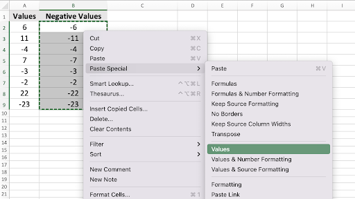
2. Using Paste Special
The Paste Special method is another way to easily convert a list to negative values. Using this method will require you to have a list that contains only positive values. If your list also contains negative values, use the steps above with the ABS method to first convert your list to absolute values.
1. The first step using Paste Special is to type -1 in a blank cell separate from your list and copy it. You can copy the value by right-clicking on the cell and selecting Copy.
2. Select your entire list of values. We’re using a short list for our example; if you have a very long list, you can click on the first cell of your list and press Shift+Command+down arrow for Mac or Shift+Ctrl+down arrow for Windows to highlight all the cells until the end of your list.
This is a useful keyboard shortcut if you’re working with large data sets.

3. Right-click on the selected cells and select Paste Special from the context menu that appears and then click on Paste Special… to open the Paste Special dialog box.

Under the Operation section in the Paste Special dialog box, select Multiply and then click on OK. This will multiply the selected range of cells with the value that you copied at the beginning, which is -1.

Now your values are successfully converted into negative values, and you can delete the -1.

If you want to change the values back to positive, you can follow the same steps again. Multiplying your values with -1 again will result in positive values. Note, however, that you won’t be back at a starting point of mixed positive and negative values.
3. Using IF function
The IF function in Excel can be just as effective in making numbers negative. For example, if column A in Excel contains your list and you want column B to contain the negative values, the following IF formula can be used in column B:
=IF(A2>0,A2*-1,A2)
If you’ve used different cells, replace “A2” with the cell containing your first value. Note that this process doesn’t require converting the starting numbers to absolute values.

Broken down into words, the formula means that if the value in column A is greater than zero (i.e. positive), multiply it by -1. Otherwise, keep the value the same. This will ensure your final list includes only negative values. If you want to convert your list back to positive values, then you can use the same formula and just change the “>” to “<” before applying the formula.
Another method is to use (VBA) Visual Basic for Applications code to first check whether each number in the selected range is positive and then convert it to a negative value. If you decide to use this method, keep a backup of your data set before running the script since the operation permanently changes the values. You can’t undo the changes once you’ve run the script.
4. Using Flash Fill
Flash Fill is a powerful feature in Excel that can automatically fill in values based on patterns it detects in your data. This feature can be used to turn a list of numbers negative, but it will need to pull from an all positive list, so start by using the ABS function.
1. Enter your data in column A that you want to convert to a negative number format.
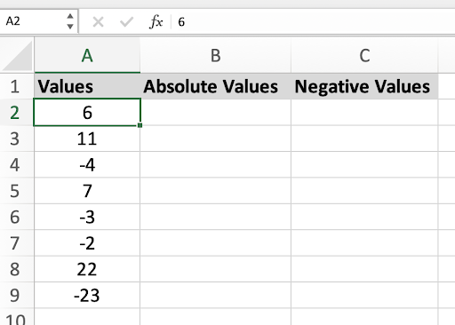
2. In an adjacent empty column, apply the ABS function as from above:
=ABS(A2)

Apply the function to the entire column.

3. Hide column A by right-clicking and choosing Hide or selecting Format/Hide.

4. In an adjacent empty column, (where you want the converted values to appear, in this case, column C), manually enter the first negative value corresponding to the first positive value.

5. Click on the cell where you manually entered the negative value (-6 in this example). Go to the Edit drop-down tab in the Excel ribbon. Locate the Fill group. Click on the Flash Fill button.

Excel will automatically detect the pattern and fill in the remaining cells in column C, converting the positive values to negative numbers.

6. Unhide column A.

5. Multiplying by -1
Using the multiplying by -1 method is an efficient way to convert numbers to negative numbers. But, like previous methods, this method requires a list of all positive numbers. We will use the ABS function to make it work.
1. Enter your data in column A that you want to convert to negative numbers.
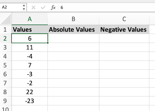
2. In an adjacent empty column, apply the same ABS function as from above:
=ABS(A2)

Apply the function to the entire column.

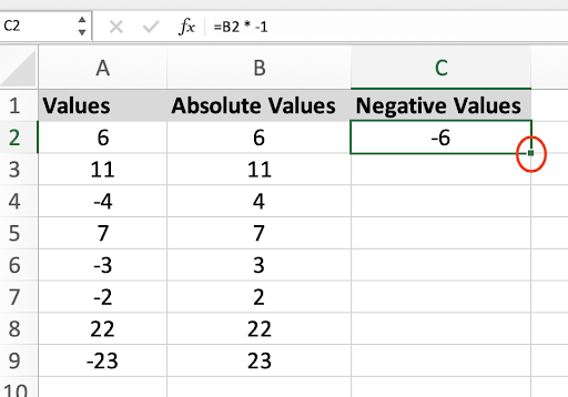
3. In an adjacent empty column (where you want the custom converted values to appear, in this case, column C), enter the formula that multiplies the corresponding cell value in Column B by -1.
In cell C2, enter the formula:
=B2*-1
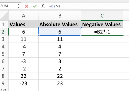
When you press enter, it will give you the negative value.

4. Drag it down to apply to the rest of the cells.
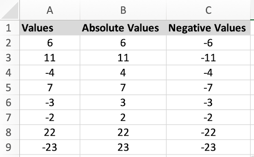
You now have a complete list of negative values.
Choosing the best method for converting numbers
You can use any of the five methods when converting a list of values to negative ones in an Excel worksheet. This can help you save time compared to changing each value individually.
Once you’ve successfully converted your list, you can revert to positive values using the same methods. These methods involve multiplying your list by -1, which will revert it to positive values. (Keep in mind that multiplying a negative by a negative results in a positive outcome.) Note, though, that if you started with some negative and some positive values, you won’t revert to your original values.
Let’s take a look at the pros and cons of each method.
The best method: The ABS function is the best option when trying to make numbers negative in Excel. The ABS function can be consolidated into one easy formula, saving time, while staying simple and easy to use.
Pro Tip: Excel formatting allows you to show negative numbers in different ways. Rather than having the minus sign, you can automatically apply parentheses or red font or both for negative numbers, popular conventions in accounting applications. Use Ctrl +1 or Format/Cells/Number to access number settings and see the choices for how negative values will appear in your spreadsheet.

You can choose between red, parentheses, or red parentheses.

If you choose just red, this is how it’ll look:

Alternatively, this is how choosing red parentheses will look:

Need help? Hire a Microsoft Excel expert
Microsoft Excel can help you accomplish your data visualization goals, but learning all the Excel formulas and Excel functions can be time-consuming. Engaging an independent Microsoft Excel expert can help you deal with your Excel needs so you can keep your focus on other important tasks of your business.
Upwork is a great platform for contracting with Microsoft Excel experts and many other freelancers to help you accomplish your business goals easily and effectively.
Search through a list of independent professionals with matching skills and schedule an interview. Making use of independent workers is a great way to get the job done by qualified professionals while freeing up more of your own time that you can put toward other business activities.

.avif)

Author Spotlight

Upwork is the world’s largest human and AI-powered work marketplace that connects businesses with independent talent from across the globe. We serve everyone from one-person startups to large organizations with a powerful, trust-driven platform that enables companies and talent to work together in new ways that unlock their potential.